Biaxial scatter plot with group medians overlaid
Source:R/plot_cluster_scatter.R
plot_group_scatter.RdCreates a biaxial scatter plot with observations colored by group assignment. Median group centroids are overlaid as large points and labeled with group names. The plot can use either raw variables (specified by the user) or dimensionality reduction components as axes.
Colour palette
When point_col is NULL, group colours are assigned automatically
based on palette_group. The "auto" strategy selects a palette by the
number of groups:
1–8 groups: Okabe-Ito — colorblind-safe 8-colour palette.
9–12 groups: ColorBrewer Paired — 12 colours pairing light and dark versions of 6 hues.
13–21 groups: Kelly's palette (optional
Polychromepackage) — 21 colours of maximum perceptual contrast (white excluded). Falls back tohue_pal()with a warning ifPolychromeis not installed.22–31 groups: Glasbey's palette (optional
Polychromepackage) — 31 algorithmically spaced colours (white excluded). Falls back tohue_pal()with a warning ifPolychromeis not installed.> 31 groups:
hue_pal()— evenly spaced hues (a warning is issued).
Set palette_group explicitly to override the automatic selection (provided
the chosen palette supports at least as many colours as there are groups).
Usage
plot_group_scatter(
  .data,
  group,
  dim_red = NULL,
  vars = NULL,
  dim_red_args = list(),
  point_col_var = NULL,
  point_col = NULL,
  palette_group = "auto",
  palette = "bipolar",
  col = c("#2166AC", "#F7F7F7", "#B2182B"),
  col_positions = "auto",
  white_range = c(0.4, 0.6),
  na_rm = TRUE,
  point_size = 2,
  point_alpha = 0.65,
  centroid_size = 3,
  label_size = 4,
  label_offset = 0.3,
  ggrepel = TRUE,
  font_size = 14,
  x_lab = NULL,
  y_lab = NULL,
  show_legend = TRUE,
  thm = cowplot::theme_cowplot(font_size = font_size) + ggplot2::theme(plot.background =
    ggplot2::element_rect(fill = "white", colour = NA), panel.background =
    ggplot2::element_rect(fill = "white", colour = NA)),
  grid = cowplot::background_grid(major = "xy")
)

plot_cluster_scatter(
  .data,
  cluster,
  palette_cluster = "auto",
  palette = "bipolar",
  ...
)
Arguments
- .data
data.frame. Rows are observations. Must contain a column identifying group membership and numeric variables.
- group
character. Name of the column in
.datathat identifies group membership.- dim_red
character or
NULL. Dimensionality reduction method: one of"none","pca","tsne","umap". IfNULL, auto-selects"none"when exactly 2 numeric vars are available, otherwise"pca".- vars
character vector or
NULL. Names of numeric columns in.datato use for the plot or reduction. IfNULL, uses all numeric columns exceptgroupandpoint_col_var.- dim_red_args
named list. Additional arguments passed to the dimensionality reduction function, overriding any defaults set by
plot_cluster_scatter. Fordim_red = "pca"these are passed tostats::prcomp()(default:scale. = TRUE); fordim_red = "tsne"toRtsne::Rtsne()(defaults:dims = 2,perplexityauto-computed,check_duplicates = FALSE,pca = FALSE); fordim_red = "umap"toumap::umap(). The data argument is always set internally and cannot be overridden. Ignored whendim_red = "none". Default islist().- point_col_var
character or
NULL. Column to use for point colour mapping. Default is same ascluster.- point_col
named vector or
NULL. Custom colours for discretepoint_col_var(named by level). WhenNULL(default), colours are chosen automatically by number of groups: Okabe-Ito for up to 8, ColorBrewer Paired for up to 12, Kelly's palette (requiresPolychrome) for up to 21, Glasbey's palette (requiresPolychrome) for up to 31, andhue_pal()for larger numbers. Ignored for continuouspoint_col_var(usecolinstead).- palette_group
character. Palette used for automatic colour assignment when
point_colisNULLfor a discretepoint_col_var. One of"auto"(default),"okabe_ito","paired","kelly","glasbey", or"hue_pal". See the Colour palette section of Details.- palette
character or
NULL. Named colour palette for the continuous point colour scale. Forwarded toplot_group_scatter(). Default is"bipolar".- col
character vector. Colours used for the continuous
point_col_varcolour scale, ordered from low to high values. Default isc("#2166AC", "#F7F7F7", "#B2182B")(blue, white, red). Any number of colours (>= 2) is accepted. Ignored whenpoint_col_varis discrete or whenpaletteis notNULL.- col_positions
numeric vector or
"auto". Positions (in [0, 1]) at which each colour incolis placed on the colour scale. Must be the same length ascol, sorted ascending, with first value0and last value1. When"auto"(default) andcolhas exactly three colours, the middle colour is stretched overwhite_range. In all other"auto"cases the colours are evenly spaced from 0 to 1. Ignored whenpoint_col_varis discrete or whenpaletteis notNULL.- white_range
numeric vector of length 2. The range of positions (on a 0-1 scale) over which the middle colour is stretched. Only used when
colhas exactly three colours andcol_positions = "auto". Also applied to divergingpalettepresets. Default isc(0.4, 0.6). Ignored whenpoint_col_varis discrete.- na_rm
logical. Whether to remove observations with missing values in the variables used for the plot axes (and dimensionality reduction, when applicable). When
TRUE(default), missing observations are removed and a message is issued showing how many. WhenFALSEanddim_redis not"none", an error is raised if any missing values are found (dimensionality reduction algorithms cannot handle them). WhenFALSEanddim_red = "none", observations with missing axis values are silently dropped by ggplot2.- point_size
numeric. Size of observation points. Default is
2.- point_alpha
numeric. Alpha transparency for observation points and legend guide. Default is
0.65.- centroid_size
numeric. Size of centroid points. Default is
3.- label_size
numeric. Font size for centroid labels. Default is
4.- label_offset
numeric. Label repulsion padding for centroid labels in cm. Default is
0.3.- ggrepel
logical. Use
ggrepel::geom_text_repelfor centroid labels. Default isTRUE.- font_size
numeric. Font size passed to
cowplot::theme_cowplot. Default is14.- x_lab
character or
NULL. Label for x axis; default uses reduction variable names.- y_lab
character or
NULL. Label for y axis; default uses reduction variable names.- show_legend
logical. Whether to show the legend. Default is
TRUE. Set toFALSEto hide the legend, as centroid labels may suffice.- thm
ggplot2 theme object or
NULL. Default iscowplot::theme_cowplot(font_size = font_size)with white background.- grid
ggplot2 layer or
NULL. Background grid added to the plot. Default iscowplot::background_grid(major = "xy"). Set toNULLto suppress the grid.- cluster
character. Name of the column in
.datathat identifies group membership. Alias for thegroupparameter.- palette_cluster
character. Alias for
palette_groupinplot_group_scatter(). See the Colour palette section of Details.- ...
Additional arguments passed to
plot_group_scatter().
Examples
set.seed(1)
.data <- data.frame(
group = rep(paste0("C", 1:3), each = 20),
var1 = c(rnorm(20, 2), rnorm(20, 0), rnorm(20, -2)),
var2 = c(rnorm(20, -1), rnorm(20, 1), rnorm(20, 0)),
var3 = c(rnorm(20, 1), rnorm(20, -1), rnorm(20, 0))
)
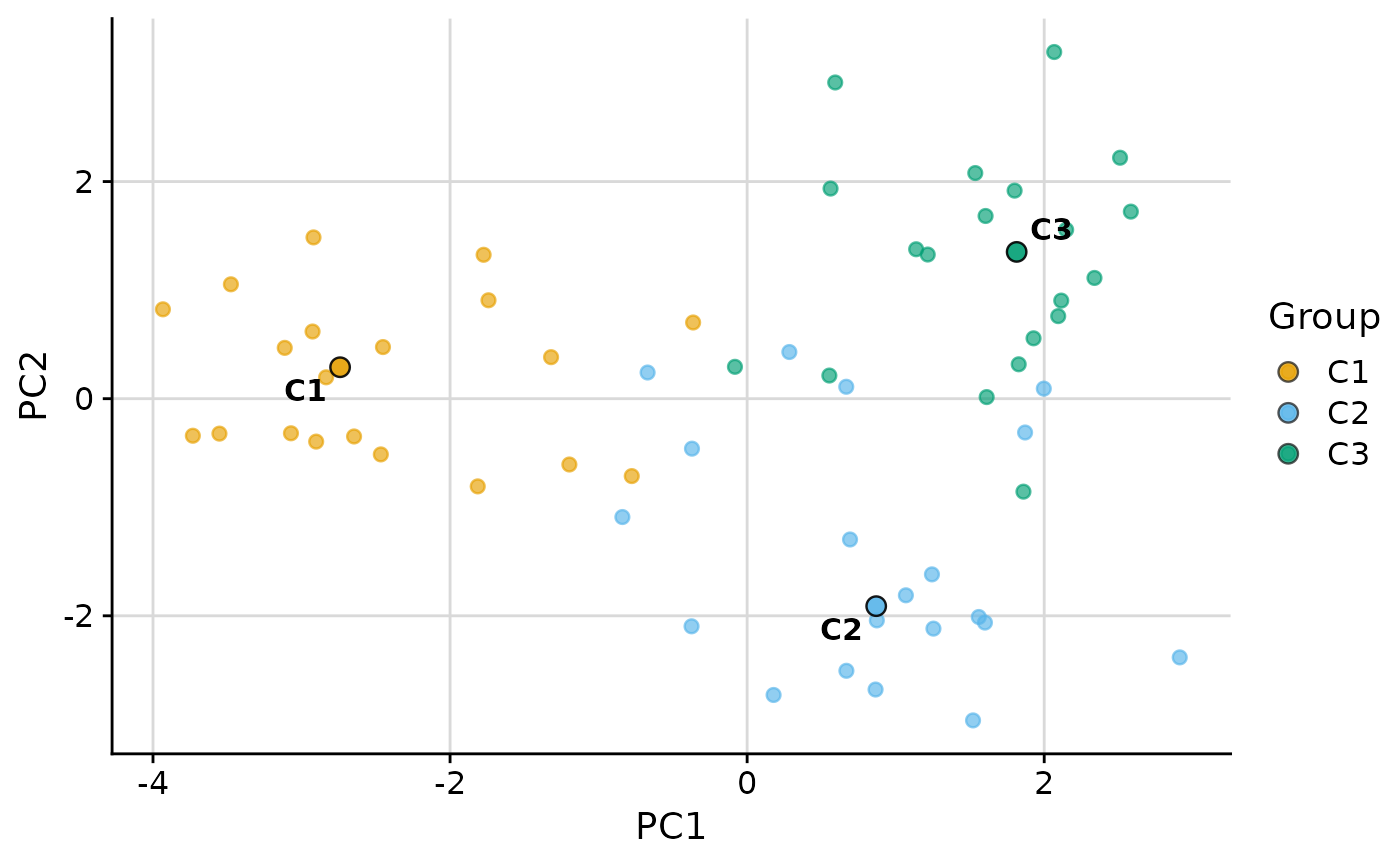
plot_group_scatter(.data, group = "group")
#> dim_red automatically set to 'pca' because more than two numeric variables are available.
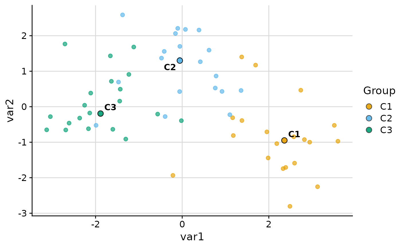
 plot_group_scatter(.data, group = "group", dim_red = "none", vars = c("var1", "var2"))
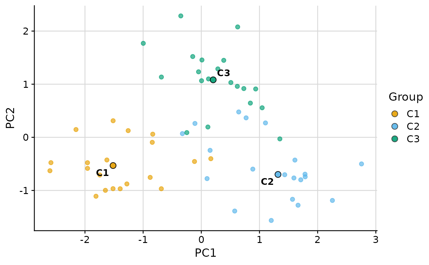
 plot_group_scatter(.data, group = "group", show_legend = FALSE)
#> dim_red automatically set to 'pca' because more than two numeric variables are available.
plot_group_scatter(.data, group = "group", show_legend = FALSE)
#> dim_red automatically set to 'pca' because more than two numeric variables are available.
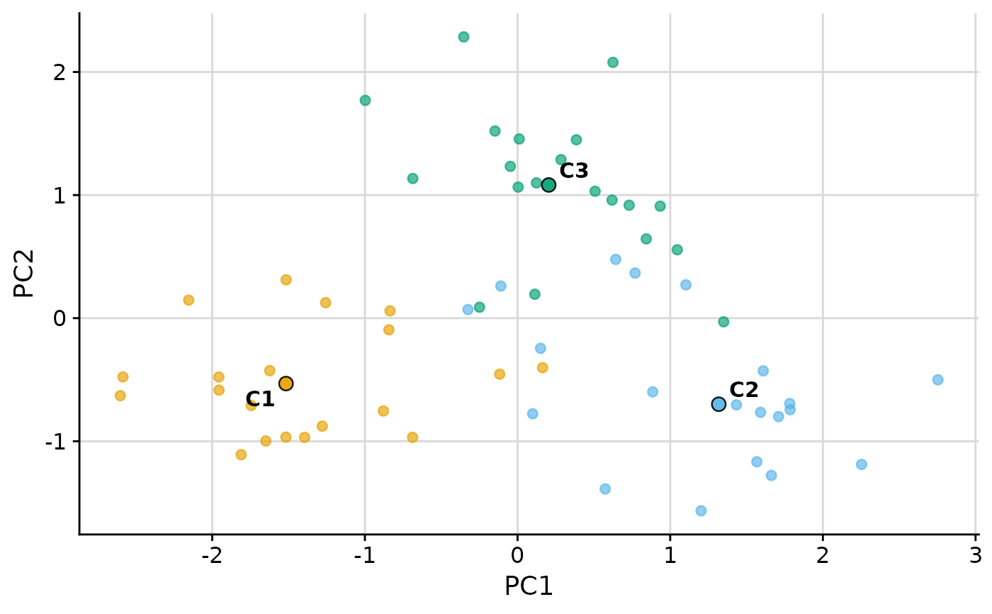 # Pass extra arguments to the dim-red function, e.g. disable scaling in PCA:
plot_group_scatter(.data, group = "group", dim_red = "pca",
dim_red_args = list(scale. = FALSE))
# Pass extra arguments to the dim-red function, e.g. disable scaling in PCA:
plot_group_scatter(.data, group = "group", dim_red = "pca",
dim_red_args = list(scale. = FALSE))